Coding a fused matrix multiplication and log-sum-exp reduction in Triton to retrieve LLM log-probabilities faster and with lower memory overhead

Motivation

In my research I have worked with methods that involve retrieving the log-probabilities of an input text from a large language model. Let me first introduce what I mean exactly and why this is useful.

Consider an input text tokenized into the sequence $t_1,\dots,t_L$. Each token is mapped to an initial embedding, forming the initial hidden-state matrix $\mathrm{HS}^0 \in \mathbb{R}^{L \times D}$. The transformer then processes these representations and produces the contextualized final hidden states

A final linear layer with weight matrix $W \in \mathbb{R}^{V \times D}$ and bias vector $b \in \mathbb{R}^{V}$ is applied to obtain the logits

Applying the softmax along the vocabulary dimension yields the probability matrix

This probability matrix encodes the model’s next-token predictions. For each position $i \in {1,\dots,L}$, the vector $P_i \in \mathbb{R}^{V}$ is a valid probability distribution (non-negative and summing to one) over the vocabulary. Its $v$-th component represents the model’s estimated probability that the next token is the $v$-th vocabulary item, conditioned on the preceding context $t_1,\dots,t_i$.

During the generation process we only compute the final probability vector to sample the new token to be appended. However, we can apply the model to a full input text and study these probabilities across tokens. This is useful in distinguishing AI-generated text (we expect these texts to score higher when passed through the LLM), and we have also leveraged them for human authorship problems.

Computational problems

The vocabulary of modern LLMs is very large (100K–300K tokens), and the matrix $P \in \mathbb{R}^{L \times V}$ becomes extremely large for long texts, especially if we batch inputs for higher throughputs. However, in our use cases, we only need the log-probability of the token that actually occurred next in the sequence; i.e., we want the sequence

If we compute these values smartly, we avoid instantiating the full probability or logit matrix in memory!

Derivations and algorithm

Now, we can consider the following equivalence:

and therefore

The first component is very easy to simplify:

The second term is a reduction across the vocabulary dimension. In other words, $\mathrm{logsumexp}(\mathrm{logits},\ \mathrm{dim}=1)$ yields a vector of length $L$, not a massive matrix. Naively, you would instantiate the full logits to compute the logsumexp, which is expensive. Instead, we can fuse the linear layer that produces logits with the logsumexp reduction in a single kernel.

Tiled matmul & online log-sum-exp

Let me first ignore the bias vector of the linear layer for simplicity now. Consider two matrices $A\in \mathbb R^{M \times K}$ and $B\in \mathbb R^{N \times K}$. We want to implement the following:

or, in non-vectorial form:

As with general matrix multiplication, we tile the matrices; each pair of tiles is handled by a tensor core. While computing tile products, we apply the exponential and maintain the running sum of exponentials across the $N$ dimension. After accumulation along $N$, we take the logarithm.

for m in range(0, M, BLOCK_SIZE_M):
    reduce_global = zeros((BLOCK_SIZE_M,), dtype=float32)
    
    for n in range(0, N, BLOCK_SIZE_N):
        acc = zeros((BLOCK_SIZE_M, BLOCK_SIZE_N), dtype=float32)
        for k in range(0, K, BLOCK_SIZE_K):
            a = A[m : m+BLOCK_SIZE_M, k : k+BLOCK_SIZE_K]
            b = B[n : n+BLOCK_SIZE_N, k : k+BLOCK_SIZE_K]
            acc += dot(a, b.T)

        reduce_global += sum(exp(acc), axis=1)
    
    C = log(reduce_global)

After dividing the algorithm in blocks, we can parallelize the program across tensor cores by blocks. Since we have a reduction dependency in both the $N$ and $K$ dimensions, we will parallelize across blocks in the $M$ dimension.

In standard matrix multiplication, you can parallelize over the tile grid in the $M$ and $N$ dimensions because each tile of the output depends only on a reduction over $K$. The $K$-dimension cannot be parallelized directly because every partial product must be accumulated in a synchronized way. In this fused matmul-logsumexp kernel, the situation is different: each $M\times N$ tile contributes to a reduction over the $N$-dimension, so $N$ also becomes a reduction axis. Because of this dependency, only the $M$-tiles are fully independent. Triton handles this by launching one program instance per $M$-tile. Each instance processes all $N$- and $K$-blocks needed for its tile.

However, there is an additional implementation detail that is critical for numerical stability. This modification is mathematically equivalent but avoids computing the exponential of large numbers:

Note that we are substracting a matrix and a vector, referring to the traditional broadcasting mechanism in PyTorch. This modification complicates our tiled implementation: we must track the online maximum across $N$-tiles and the sum of translated exponentials. This can be seen as a reduction with the following operator:

The initial sequence would be transformed by the map

We are now ready to present the full algorithm:

for m in range(0, M, BLOCK_SIZE_M):
    reduce_global = zeros((BLOCK_SIZE_M,), dtype=float32)
    max_global = full((BLOCK_SIZE_M,), float('-inf'), dtype=float32)
    
    for n in range(0, N, BLOCK_SIZE_N):
        acc = zeros((BLOCK_SIZE_M, BLOCK_SIZE_N), dtype=float32)
        for k in range(0, K, BLOCK_SIZE_K):
            a = A[m : m+BLOCK_SIZE_M, k : k+BLOCK_SIZE_K]
            b = B[n : n+BLOCK_SIZE_N, k : k+BLOCK_SIZE_K]
            acc += dot(a, b.T)

        max_block = max(acc, axis=1)
        acc = exp(acc - max_block[:, None])
        reduce_block = sum(acc, axis=1)

        # Update global values
        max_global_new = maximum(max_global, max_block)
        reduce_global = (
            reduce_global * exp(max_global - max_global_new) +
            reduce_block * exp(max_block - max_global_new)
        )
        max_global = max_global_new
    
    C = max_global + log(reduce_global)

The full Triton code is available at pablomiralles22/fused-matmul-logsumexp, and you will find a good description and instructions on how to use it on the README file.

Benchmarking

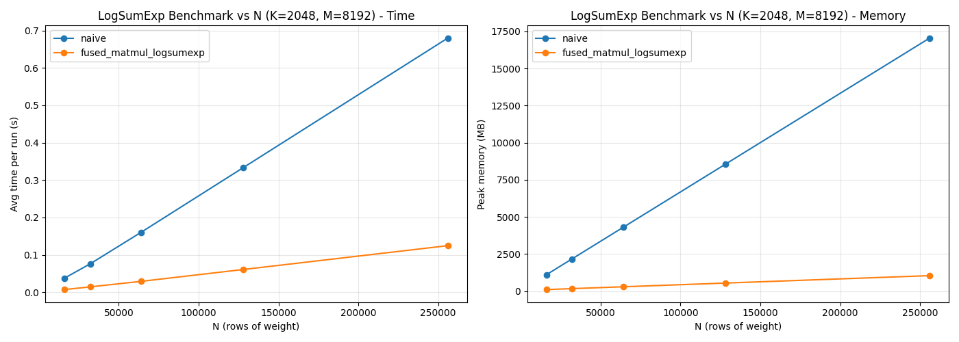
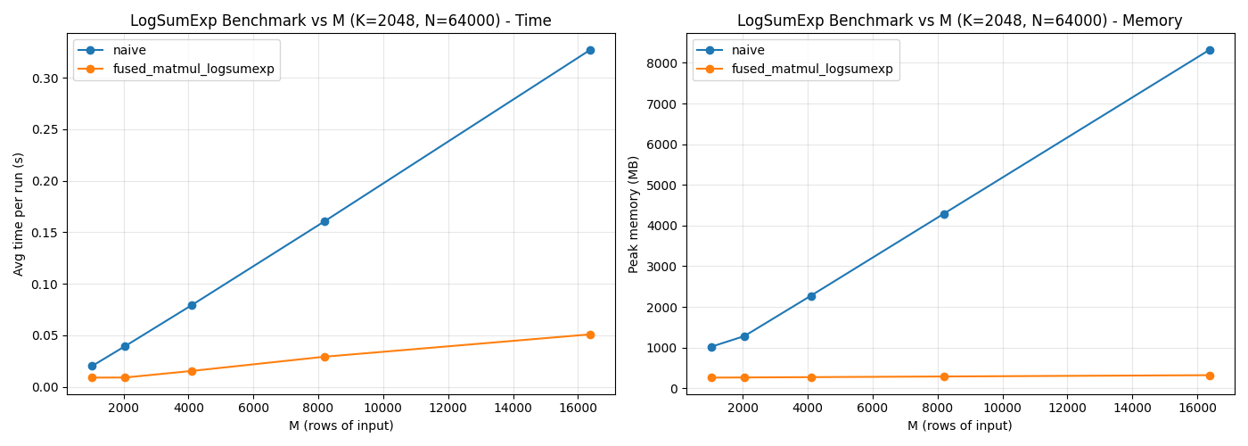
Consider an input matrix $X\in \mathbb R^{M \times K}$, a weight matrix $W\in \mathbb R^{N \times K}$, and a bias vector $b\in \mathbb R^{N}$. The following plots show execution time and peak memory for varying $M$ and $N$, comparing the fused implementation to a naive baseline: